The 10% rule
Unless you have already spent time optimising your code, it is virtually certain about 10% of the code is responsible for essentially all the delay you encounter in getting your results. This is true of all programming tasks – whether using Mathematica or some other language such as C, Java, or Fortran. It is easy to waste time optimising some of the code from the 90% and see no improvement whatsoever! Therefore, the first task is to find the part of your code that is consuming the time. Assuming that your program can run on a range of data sets of various sizes, you should try to pick an example that takes – say – 30 seconds to run. You will end up running the code many times, so you don't want something that takes too long, but equally you need to be able to study that time delay.
The simplest way to identify the slow part of your code, is to add Print statements. This may sound crude, but if you can reach a point where two Print statements bracket a small chunk of code that takes a significant time to execute, that is real progress. Be ready for some surprises – for example, some file formats can be Exported/Imported far more efficiently than others, and this often changes with new versions of Mathematica.
I believe the Wolfram Workbench can also help to identify the hotspots in your code in a slightly more formal way called profiling. As yet, I have not explored this product – I guess I am not a great fan of IDE's in any programming language, this may be a function of my age!
Avoid nasty surprises!
The speed of a Mathematica calculation can be rather hard to predict, so it is important to avoid the trap of developing a complex algorithm with miniature development data sets, only to discover when it is too late that your calculation is far too slow when applied in earnest.
The curse of generality
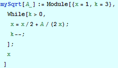
Mathematica can manipulate a wide variety of objects, such as integers, reals, fractions, surds, and symbolic expressions. Sometimes this generality can create problems, and quite straightforward code can seem to execute unbelievably slowly. Consider the following loop, which applies three cycles of Newton's method for approximating a square root:

This definition works fine with real data, but look what happens if it applied to exact data:
![]()

When you look at this expression it is hardly surprising that this is rather inefficient – in effect, we have forced Mathematica to perform a huge algebraic calculation! Of course, this problem is easy to rectify once it is recognised, the insidious thing is that the expression might be generated and only subsequently reduced to a number. The only evidence that something unusual was happening would be the time required to obtain the result.
Notice that in the above definition we used a loop count of 3. In a more realistic definition a larger loop count would be used, or the FixedPoint function might be used. In that case the calculation would probably just hang!
Functional programming
Open any Mathematica book and you are bound to read about the virtues of functional programming. There is indeed value in functional programming, but I want first to add a little perspective. Here is a trivial example of some functional programming – applying the function Sin to a list of numbers:
![]()
![]()
or, using the fact that Sin has attribute Listable:
![]()
![]()
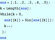
We are told that constructions like that are more efficient than a loop (based perhaps on While), and indeed, this is the case. However, it is instructive to think about exactly why this is so. At first glance, you might think that either of these constructs allow all the Sin calculations to get done in parallel, however, this is not true, even if you are using a multi-core CPU! Strangely enough, ultimately, Mathematica computes all those trig functions in a loop – because it has to use the instructions available in your computer architecture. If you could translate that loop back into Mathematica code, it would look remarkably like the inefficient code that we are told not to use:

![]()
The loop might spin in the opposite direction, but the essence of the code would be as shown.
In order to understand this paradox, it is necessary to understand that when Mathematica executes a loop such as the one above, it has to do far more work than simply performing the required calculations. There is a big overhead attached to each step. Consider just one line:
![]()
Executed as a machine instruction to increment the value of an integer, this might take 1-3 instructions, depending on the architecture. On a modern machine, that would take about 1 nanosecond. However, Mathematica must first determine if 'k' has a value (otherwise there is an error), and what sort of value it has – it might be a real, or a rational, or even symbol. It also has to ensure that the built in 'Decrement' function has not been user modified. In addition, the concept of an integer is not quite the same to Mathematica as it is to the CPU. Mathematica integers never overflow (except for truly gigantic numbers that fill all of memory), and so Mathematica has to test for overflow and change the representation of the integer if necessary.
All of this work takes time and will happen on each turn of the loop. The point is that each individual step of a calculation carries an overhead like this, so if you can do a Mathematica calculation in a small number of large steps (such as the above Map function call) then you will get better performance. Functional programming offers little if any speed advantage in conventional compiled programming languages, because the variables have pre-declared types, and the programmer is responsible for avoiding overflow situations.
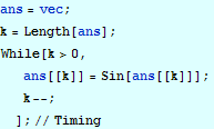
Put another way, in the context of Mathematica, functional programming is a good way to reduce the number of individual steps in a calculation and thereby reduce the associated overhead. Let us now examine how big this gain can be. To do this, we really need a longer vector if numbers:
![]()
![]()
![]()
![]()
![]()

![]()
In the above calculations I have adjusted the expressions slightly to throw away the results numbers), and I also had to adjust the size of the array so as to get reasonable timing information.
Notice first that using the Listable attribute of Sin is over 12 times more efficient than using Map! The main lesson to learn from this seems to be that Mathematica constructs can vary in performance quite remarkably, and it pays to do some experiments.
The explicit loop is 35 times as expensive as even the Map construct – and illustrates the benefit of avoiding explicit loops where possible. Note that Sin is a built-in function. If instead we used a complicated user-defined function in either construct, then the relative gain might be much less. Functional constructions can become very complicated in situations in which, perhaps, not all values of 'k' are to be treated the same way – reasonable judgement is called for.
Packed arrays
Let us re-run the first two experiments with one – seemingly insignificant – change. We rplace one of the
![]()
![]()
![]()
![]()
![]()
![]()
These timings are substantially greater than before, and do not seem to reflect the actual elapsed time. This is almost certainly due to the fact that substantial page-swapping is going on. This is a dramatic illustration of yet another feature of Mathematica programming.
In early versions of Mathematica, a List was simply a Mathematica data structure like any other, with 'List' as its head. For many examples of lists, this is still true, but homogenous arrays (in one or more dimensions) of reals, integers, and complex numbers can also be stored as packed arrays, which resemble arrays in Fortran or C. Such arrays are much more compact, and can also be accessed at very high speed. The system can choose to convert between its two representations of lists in a totally silent way, because the results of no ordinary calculations depend on this representation – only the efficiency varies. Note in particular, that just because a particular list is elligible to be packed, does not necessarily mean that it will be. Some functions, such as 'Table', seem to pack their result where possible, but it is easy to create an array that is unpacked but could be packed.
The large vector in the previous example was unpacked when the following statement turned it into a mixture of reals and integers.
![]()
The following statement could be used to fix that:
![]()
This uses 'N' to make the array homogenous once more, followed by Developer`ToPackedArray, which packs its argument if possible. It is also possible to test an array to determine if it is indeed packed:
![]()
![]()
Even though these functions are in Developer` context, they are vital for anyone who wants to optimise Mathematica code involving large arrays.
Conclusion
The above is really just an introduction to the complex matter of optimising Mathematica code. If you feel your Mathematica code needs speeding up, I may be able to help. I will look at your code and attempt to improve its performance. Only if I succeed, will I request a consultancy fee in return for the enhanced code.
Obviously, I may decide that I do not wish to work with particular pieces of code for any of a variety of reasons, but in that case you will only have wasted the electricity required to send me an e-mail!


